Resurrecting this blog. Recently I have been giving lectures on hyperbolic geometry to my students including student trainees. The lectures allow me to brush up on basics of hyperbolic geometry for upcoming conference and also to help the trainees do their mini projects. I begin with the models of hyperbolic plane.
Hyperboloid Model
Everyone knows the unit (two-) sphere whose equation is 

If one changes the sign in one variable of the sphere-equation, 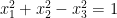

If one changes the sign of the constant on the right hand side, 

These disconnected pieces remind us the hyperbola curves we plotted in schools 

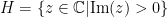
One should also mention the other possibility from the two-forms of the hyperboloid earlier, the one with zero on the right hand side, giving a double cone reminiscent of the light cones in relativity.

These null surfaces are the asymptotes of the hyperboloids (very much like the asymptotes of the hyperbola).
Returning to the double-sheeted hyperboloid; let us restrict to the positive sheet namely

it gives the hyperboloid model of the hyperbolic plane. The surface can be parametrised in ‘angular’ coordinates much in the same way as the sphere via

which leads to 


Using this bilinear form, one could actually form the metric on 


Beltrami-Klein Model
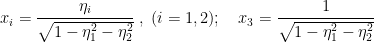
In the hyperboloid model 


The point 

Thus under this project the hyperboloid
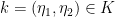
one can get the hyperboloid differentials in terms of these new coordinates as
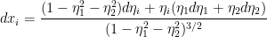
for 

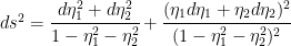
Hence the metric for the B-K disk to be
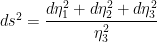
Hemispherical Model
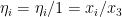
Another interesting model is to project the points of hyperboloid further to a hemisphere 

The point 


Hence, the hemisphere model of the hyperbolic plane. Note that this (hemi-)sphere has a different metric inherited from the hyperboloid i.e.
Poincare Disk Model
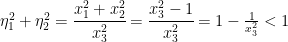
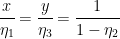
Using the hemisphere model, we can now make a stereographic projection from 


The relation between these coordinates are given by the similar triangle relations

One can work backwards (easier) to show that the Poincare disk metric
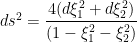
is equivalent to the metric of the hemisphere model earlier.
Upper Half-Plane Model
Now in the Poincare disk, we use the stereographic projection from 


The relation again between these coordinates are given by the similar triangles:
Unlike the earlier stereographic projection that squashes the hemisphere into a bounded (Poincare) disk, the present projection gives an unbounded plane due to the point 


This upper half plane can be realised as
This is probably one of the most convenient model to work with. It can be realised as a homogeneous space. Consider the action of 

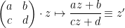
where 


It would seem like that each point on 


Thus in general for each point there will be effectively an (conjugated) 

In the next few forthcoming posts, we will investigate this model of the hyperbolic plane further
References
- Pages from http://en.wikipedia.org/wiki/Main_Page
- S. Katok, “Fuchsian Groups, Geodesic Flows on Surfaces of Constant Negative Curvature and Symbolic Coding of Geodesics”, (http://www.math.psu.edu/katok_s/cmi.pdf)
- J.W. Cannon, W.J. Floyd, R. Kenyon & W.R. Parry, “Hyperbolic Geometry” (http://www.math.brown.edu/~rkenyon/papers/cannon.pdf)
- R. Hayter, “The Hyperbolic Plane – A Strange New Universe” (http://www.maths.dur.ac.uk/Ug/projects/highlights/CM3/Hayter_Hyperbolic_report.pdf)
- J. Hilgert, “Maass Cusp Forms on
