I will leave Bengtsson & Zyczkowski book for awhile to look into dynamical systems and nonlinear dynamics, a topic I covered in my talk in India.
The subject of dynamical system is very broad (either from physics or mathematics), which makes it hard for a beginner (me) to survey the subject. It is only better for me to explain why am I interested in this area. The procedure of quantization often begins with classical (dynamical) systems of which a major interest is in quantizing (a particle system on) nonlinear configuration spaces. Most of the time we treat the nonlinearities intrinsically by adopting the appropriate canonical variables to be quantized (or quantization by constraints). Some of these nonlinear systems can be chaotic classically such as particles on hyperbolic surfaces (see review article “Chaos on the Pseudosphere” by Balasz and Voros or “Some Geometrical Models of Chaos” by Caroline Series) and it is often pondered how such behaviour translates into the quantum regime. My original concern in this topic is mostly how complex topologies of hyperbolic surfaces get encoded in quantum theory. We will defer such discussions to a later time.
What is a dynamical system? There are three ingredients to a dynamical system:
- Evolution parameter (usually time) space
 ;
;
- State space
 ;
;
- Evolution rule
 .
.
Note that can either be  or
or  , for which the former is called discrete dynamical systems where evolution rule is usually difference equation, while the latter is called continuous dynamical systems with the evolution rule described by ordinary differential equation. One can consider to discretize the state space itself to give cellular automata with their update rules (see also graph dynamical systems). Perhaps the most famous cellular automata (CA) is Conway’s Game of Life build upon a two-dimensional (rectangular) lattice whose update rule is given by
- Any live cell with fewer than two live neighbours die (underpopulation).
- Any live cell with two or three live neigbours live.
- Any live cell with more than three live neighbours die (overpopulation).
- Any dead cell surrounded by three live neighbours live (regeneration).
Fascinating configurations can be constructed by such simple rules. Even simpler is the elementary 1-dimensional CAs for which Wolfram has classified according to their update rules: rule 0 to 255 ( rules). It was proven by Cook that rule 110 is capable to be a universal Turing machine. Note in the above CAs, there are only two states (live or dead). One can generalise the number of states to go beyond two e.g. CA with three-valued state (RGB) can be used in pattern and image recognition (see e.g. https://www.sciencedirect.com/science/article/pii/S0307904X14004983).
One can further make abstract the notion of dynamical system as done by Giunti & Mazzola in “Dynamical Systems on Monoids: Toward a General Theory of Deterministic Systems and Motion” (see also here). We will not pursue this but instead mention two other cases normally not classed as dynamical systems.
I would like to add further to the above some dynamical systems encountered in (theoretical) physics that ought to be differentiated from the classes above. First, systems whose equations are given by partial differential equations i.e. those with differential operators of not only with respect to time, but also with respect to space. Most notable example is the Navier-Stokes equation that governs fluids. At this point, one should even mention about relativistic systems whose evolution parameter might not even be separably identified from spatial coordinates. Relatively recently, techniques of (conventional) dynamical systems have found its way into cosmology via long-term behaviour of cosmological solutions and reducing the full Einstein equation (pdes) to simpler ones. See the book of Alan Coley or the book of Wainwright & Ellis. See also the articles of Boehmer & Chan and Bahamonde et al. (published version here). It is interesting to note the author of former article Dr. Nyein Chan was in Swinburne University, Sarawak Campus before. He has probably returned to his home country Myanmar (his story can be read here).
To discuss geometry of dynamical systems, I make extensive use of the notes by Berglund (arXiv: math/0111177). To start, dynamical systems are equipped with a first order ODE describing the dynamical equation:
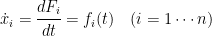
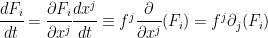
where  is a function on the state space . Using chain rule, one can rewrite this equation as
 .
.
Note that  can now be treated as a vector field (as one does in usual (local) coordinate-based differential geometry). Vectors field (despite its local coordinatization whose transformation law is known) encodes geometric information of the state space it lives on. The easiest way to see this is the exemplification of the hairy ball theorem by the statement one can’t comb the hair of a coconut. On the other hand, one can do so on the torus (surface of a doughnut). Technically this is due to the nonvanishing Euler characteristic of the sphere( and in the case of the torus, it vanishes).
The standard example of a dynamical system comes from mechanical systems (say, one particle obeying Newton’s laws). However Newtonian equations for such systems are second order ODEs. This simply implies that the mechanical state should be a pair of variables, say of position and momenta  forming the phase space
  . Formulating the mechanical system as Hamiltonian mechanics, one can rewrite the Newtonian equations of motion as two sets of first order ODEs known as Hamilton’s equations:
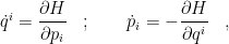
where  is the Hamiltonian of the system. It is convenient to rewrite this equation using another algebraic structure known as Poisson bracket which is defined as
 .
.
Then one can rewrite Hamilton’s equations as
 .
.
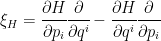
The convenience is that the dynamics is contained in the algebraic form of Poisson bracket. Thus, studying the Poisson bracket structure is equivalent to studying the dynamical structure. One can further ‘geometrize’ this algebraic structure by considering the vector fields on the phase space  and
and  and the Hamilton’s equation as
 ,
,
where  is a covariant antisymmetric tensor known as the symplectic form and
 .
.
The manifold (space) equipped with the symplectic form is known as the symplectic manifold. With the Poisson bracket replaced by the symplectic form, one can simply study the properties of the symplectic form to know about the dynamics. Finding symmetries preserving the symplectic form has become the basis of (some) quantization procedure.
The motivation to study dynamical systems is to learn about chaotic dynamical systems. The word chaos conjures images like the ones below (a favourite picture from Bender & Orszag book and a billiard in )
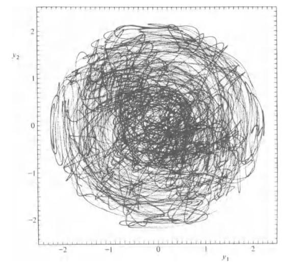
Source: Bender & Orszag, “Advanced Mathematical Methods for Scientists and Engineers” (McGraw Hill, 1978) Fig.4.23 on page 191.
However, the iconic diagram one associates with chaotic dynamical system is that of the two winged Lorenz butterfly diagram (later), which I thought it had structures. In such a system it was the sensitivity of initial conditions for the orbits traversed that played a characteristic role. The orbits above are perhaps closer to a different concept of the ergodic hypothesis. How sensitivity of initial conditions have been called chaotic is quite interesting. A more mundane name for the whole subject is nonlinear dynamics which is used before the term chaos got popular.
So how does one put some useful handles to such systems with complicated behaviour? One begins by looking for simple solutions i.e. stationary solutions. Recall  and
and  . (Note: at times, I will not write out the indices and should be understood contextually.) A stationary solution is the one that obeys
  i.e. doesn’t change with time. Of related interest are fixed points
  such that
  ; also called equilibrium points. Points for which
  are called singular points of the vector field
  ; also called stationary orbits.
We can now explore solutions nearby the equilibrium point  for which

where
 ,
,
i.e. linearizing the solutions with the higher order terms are assumed to be bounded by some constant. In the linear case ( ), one has
 .
.
Thus, one can see that the eigenvalues of  of
of  will play in the important role of long-term behaviour of the solutions.
To take advantage of this fact, one can use projectors  to eigenspace of to study the behaviour of equilibrium points. Construct projectors to sectors of eigenvalues
 .
.
and define subspaces
 ;
;
 ;
;
 ,
,
which are called respectively unstable subspace, stable subspace, and centre subspace of and they are invariant subspaces of  . With respect to these spaces, one can actually classify the equilibrium points. The equilibrium point is a sink if
  ; a source if
  ; a hyperbolic point if
  ; and an elliptic point if
  . Note that one has a richer variety of equilibrium points than the one-dimensional case simply because there are more ‘directions’ to consider in higher-dimensional cases (characterised by the eigenvalues of ). To illustrate this, we consider the two-dimensional case with two eigenvalues
  (borrowing diagram from Berglund):
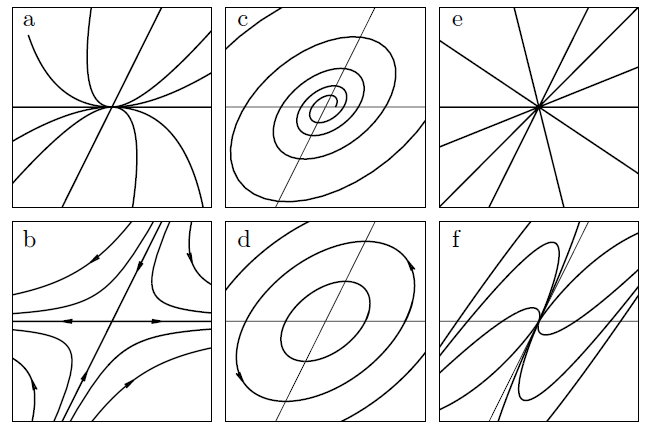
Case (a) refers to a node in which  (arrows either pointing in or out). Case (b) is a saddle point in which
  . Cases (c) and (d) happen when
  and hence giving rotational (or oscillatory motion in phase space). Cases (e) and (f) are more complicated versions of nodes when there are degeneracy of eigenvalues (please refer to Berglund for details). At this juncture, it is appropriate to mention the related concepts of basins of attraction which appear in chaotic dynamics literature. Particular one has the concept of strange attractor, arising from the fact that while is assumed continuous, the vector field may be singular at some points and thus giving rise to space filling structures known as fractals (see this article).
To proceed beyond the linear case, one needs extra tools namely the Lyapunov functions (often in the form of quadratic forms) that set up level curves over which phase space trajectories can approach or cross and help characterise stability of equilibrium points in general. The Lyapunov functions are those functions  such that
 for
for  in the neighbourhood of ;
- its derivative along orbits
 is negative showing is stable.
To illustrate this, we borrow again a diagram of Berglund to show how phase space orbits approach or cross the level curves of .
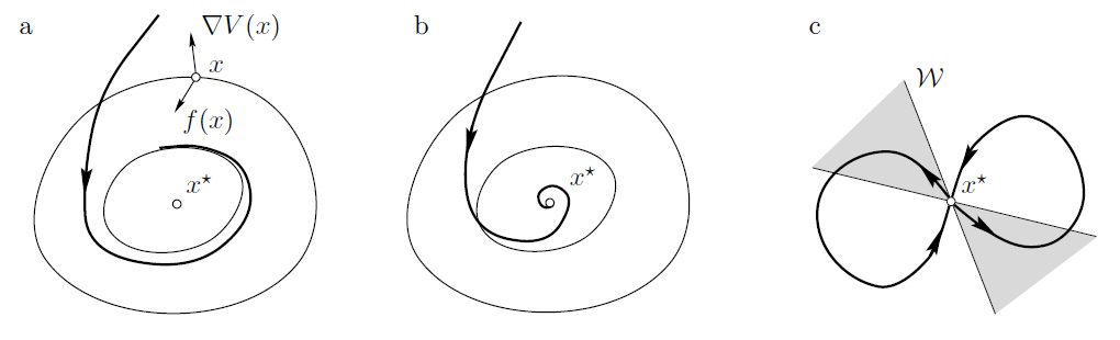
Cases (a) and (b) are respectively the stable and asymptotically stable equilibrium points where trajectories cut the level curves in direction opposite to their normals. Case (c) is the case the unstable equilibrium point generalizing the linear case where orbits may approach the point in one region and moves away in another region. Such orbits are called hyperbolic flows. This is essentially the case of interest. Note in particular if one reverses the arrows, there is invariance of the two separate regions of stable and unstable spaces and the special status of hyperbolicity.
One can now state a result known in the literature i.e. given a hyperbolic flow  on some
  , a neigbourhood of hyperbolic equilibrium point , there exists local stable and unstable manifolds
 ;
;
 .
.
For further technical details, consult Araujo & Viana, “Hyperbolic Dynamical Systems” (arXiv:0804.3192 [math.DS]) and Dyatlov, “Notes on Hyperbolic Dynamics” (arXiv:1805.11660 [math.DS]).
Examples for which hyperbolic flows are known are the cases of geodesic flows on negatively curved (hyperbolic) surfaces and billiard balls in Euclidean domains with concave boundaries (see Dyatlov). Hyperbolicity then becomes a paradigm for structurally stable ergodic system as discussed by Smale in 1960s (see Smale, “Differentiable Dynamical Systems“, Bull. Amer. Math. Soc. 73 (1967) 747-817). While this is so, unknown to the mathematicians then, E. Lorenz discovered a dynamical system that was neither hyperbolic nor structurally stable (see Lorenz, “Deterministic Nonperiodic Flow“, J. Atmosph. Sci. 20 (1963) 130-141). A new paradigm is needed to account for such systems. However, we will defer this discussion to a future post.
 be two sets. A mapping
  to
to  denoted as
  is a subset of
  such that for every
  , there is a unique
  for which
  i.e.
i.e. .
. or
or  . The element
  is called a transformation of
  is also called the graph of the function
  defined by
 . Then the inverse image
  is
is .
. does not exist and hence giving the empty set.
 . The inverse image of
  is
is ,
, , its inverse image is
 .
. of
of  . Note that
 with
with
 , where
  is said to have
  arguments. One can further generalize this by making each argument coming from different spaces i.e.
 ,
, for some
  . An important map of this nature is the projection map
 . The projection
  essentially gives the ith component of the domain.
 and
and  are maps, then the composition map
  is defined by
 .
. and
and  are maps. Then
 .
. .
. .
. i.e.
i.e. .
. has the property
 .
. , the bijective map
  is called a transformation or permutation of
  where
where .
. .
. .
. are bijections (with codomain and domain), then so is
  with the inverse
 .
. and
and  .
. ,
, .
. as follows:
 .
. which are by definition characteristic functions of (other) subset
  .
. are in one-to-one corresponding of all possible maps
  .
. be an equivalence relation on a set
  from the set
  can be given by
![\varphi(x)=[x]_R](https://s0.wp.com/latex.php?latex=%5Cvarphi%28x%29%3D%5Bx%5D_R&bg=ffffff&fg=000000&s=0&c=20201002) .
. can be introduced via transformation/permutation
  or
or  :
: and
and 
 , then
 are surjective
 is surjective;
 be maps. Then
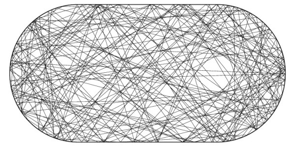
 ,
,  can be combined as
 will still belong to the set. Should be stated here that the fact that we have the linear addition of points necessitates the space it belongs to is a linear space (hence the use of
  ). One could in fact remove the requirement of a special point (say, the origin) in vector spaces and consider the embedding space being simply an affine space with linear addition operation still in place.
 and that the convex combination involves a real parameter
  . One question comes to mind is how this generalizes to complex linear spaces (as in quantum theory). Found a paper, “
 and embed the unit
  to form
  in the convex combination. This will imply the loss of ordering. However they also mention the use of inner product of elements of the embedding space to form the necessary reals if required.
![[0,1]](https://s0.wp.com/latex.php?latex=%5B0%2C1%5D&bg=ffffff&fg=000000&s=0&c=20201002) and it obeys additivity property
and it obeys additivity property ,
, . One can extend this to continuous labelled events and the sum extends to an integral. Generalizing even further one can let the measure be defined for (Minkowski) sum of convex sets (say,
  ) in such a way that they obey
  .
. .
. –convex measure. The special case of
  gives
gives
 .
. (typically density matrices if the Hilbert space is finite-dimensional). Generally density operators
  ;
; ;
; .
. (twice projection has the same effect as the first single one).
 . Hence the relation of convex geometry to quantum theory. While mixed states are the more general form (which includes pure ones), it is normally the case that one needs to define what the pure states are first (through some procedure, say, quantization). The other interesting point is that the expression of the mixed state in terms of pure state is not unique; physically translating as two statistical mixtures with same statistical averages cannot be distinguished. Mielnik likened this to be similar to the use of local coordinates in Riemannian geometry and promoted convex geometry as the geometry for (even a generalised) quantum mechanics – see Mielnik, “
 and
and  . A subset
  ,
, lie in
  -face is a facet. Given the set of all feces of a convex body, one can form a partial ordering i.e.
  if face
  is contained in
  . This leads to another idea: partial ordering is the essential ingredient to form a logic, allowing what statements can be made. Thus convex geometry is related to the idea of quantum logic proposed much earlier and this is discussed in Mielnik, “
 obeying Maxwell’s equations. It is convenient to introduce scalar and vector potentials
  to help solve such that
 i.e.
i.e.
 are defined modulo phase factors (see B. Felsager,
 but yet retains the canonical commutation relations implying a form of gauge symmetry. See
 where
where  is the symplectic potential often given as
  (see P. Libermann & C.-M. Marle,
  .
. . (see Ciaran Hughes, “A Brief Discussion on Gauge Theories” for a brief introduction,
 giving Klein-Gordon equation
  .
. giving Dirac Equation
  .
. giving Maxwell equation
  .
. , one consider the transformations by a (global) phase factor:
 .
. group element. The free fermion Lagrangian above is invariant under this global phase transformation.
 with the Lagrangian
 .
. transformations
 .
. sending
  to
to  . Then the Lagrangian transforms as
 such that the derivative transforms as needed:
 .
. ,
, is an element of
  is the (gauge) coupling constant. Note that the ambiguity of the gauge fields (potentials) is still there with the gauge field transforms as
 .
. (summed over generators of the Lie algebra
  . This is given via the field strength tensor
![F_{\mu\nu}= F^a_{\mu\nu} T^a=[D_\mu,D_\nu]](https://s0.wp.com/latex.php?latex=F_%7B%5Cmu%5Cnu%7D%3D+F%5Ea_%7B%5Cmu%5Cnu%7D+T%5Ea%3D%5BD_%5Cmu%2CD_%5Cnu%5D&bg=ffffff&fg=000000&s=0&c=20201002) .
. and that
 .
. as such term will break the gauge invariance of the Lagrangian.Hence at this stage, gauge fields are considered massless.
 gauge theory. The complication is that the gauge fields that mediate the weak interaction are massive (the
  particles) and hence must include a further ingredient which is the Higgs field and the idea of spontaneous symmetry breaking, which is the subject of the conference mentioned earlier. What one sees as weak interaction and electromagnetic interaction are really remnants of the
  . See J. Hucks, “
 which is understood as the square root of the Laplacian
  i.e.
i.e.  . If it is one dimensional with
  , this would have been straightforward. For more than one dimension, this is nontrivial – what is the square root of say
  ?
? -deformed numbers
 are integers. By making
  , one then has the alpha-deformed addition
 . For more cases of the integer, it is


 i.e. it works like the ordinary derivative with numbers replace by the deformed numbers. One could generalise this further to power series functions. For instance the
 and form the


 where
where  is the current density of the loop. The current may be carried by a charged particle orbiting in a loop. From the formula given, the magnetic moment is then proportional to its angular momentum.
 , then its magnetic moment is
 is the Bohr magneton and
  is the gyromagnetic factor (dimensionless magnetic moment). Now according to Dirac’s theory,
  but this quantity receives corrections from QFT which can be written as
 can be written as a (divergent) power series of the fine structure constant

